45 direct label excel charts
Directly Labeling Excel Charts - PolicyViz Stephanie's showed two ways to directly label a line chart in Excel. Method #1 used the new labeling feature in Excel 2013. In Method #2, she inserted text boxes in the graphic; this approach would work in just about any version of Excel. Let me offer two alternative ways to directly label your chart. Method #1 › databases › questiaQuestia - Gale Individual subscriptions and access to Questia are no longer available. We apologize for any inconvenience and are here to help you find similar resources.
Custom Chart Data Labels In Excel With Formulas - How To Excel At Excel Select the chart label you want to change. In the formula-bar hit = (equals), select the cell reference containing your chart label's data. In this case, the first label is in cell E2. Finally, repeat for all your chart laebls. If you are looking for a way to add custom data labels on your Excel chart, then this blog post is perfect for you.

Direct label excel charts
How to Change Text or Label Direction in Excel Chart - YouTube In this video, you will learn how to change the direction of text or label in excel charts. Data Labels in Excel Pivot Chart (Detailed Analysis) Add a Pivot Chart from the PivotTable Analyze tab. Then press on the Plus right next to the Chart. Next open Format Data Labels by pressing the More options in the Data Labels. Then on the side panel, click on the Value From Cells. Next, in the dialog box, Select D5:D11, and click OK. Excel Charts: Dynamic Label positioning of line series - XelPlus Select your chart and go to the Format tab, click on the drop-down menu at the upper left-hand portion and select Series "Budget". Go to Layout tab, select Data Labels > Right. Right mouse click on the data label displayed on the chart. Select Format Data Labels. Under the Label Options, show the Series Name and untick the Value.
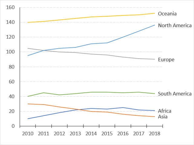
Direct label excel charts. › us-en › shopHP® Computer and Laptop Store | HP.com Find a great collection of Laptops, Printers, Desktop Computers and more at HP. Enjoy Low Prices and Free Shipping when you buy now online. 7 steps to make a professional looking line graph in Excel or ... The chart title should usually be the largest font (and can be in bold), the direct labels on each line and explanatory text next largest, and the axis labels can be slightly smaller. Use color to focus attention By default each line is a different color based on the order of colors in the color theme. Excel Chart Data Labels-Modifying Orientation - Microsoft Community Excel Chart Data Labels-Modifying Orientation. The chart layout tab has been absorbed into other areas in Excel 2016. I cannot figure out how to change the orientation of the data labels on the axes.... (tilt, horizontal, vertical). Any help is appreciated! Creating a chart with dynamic labels - Microsoft Excel 2016 For the existing chart, do the following: 1. Right-click on the chart and in the popup menu, select Add Data Labels and again Add Data Labels : 2. Do one of the following: For all labels: on the Format Data Labels pane, in the Label Options, in the Label Contains group, check Value From Cells and then choose cells:
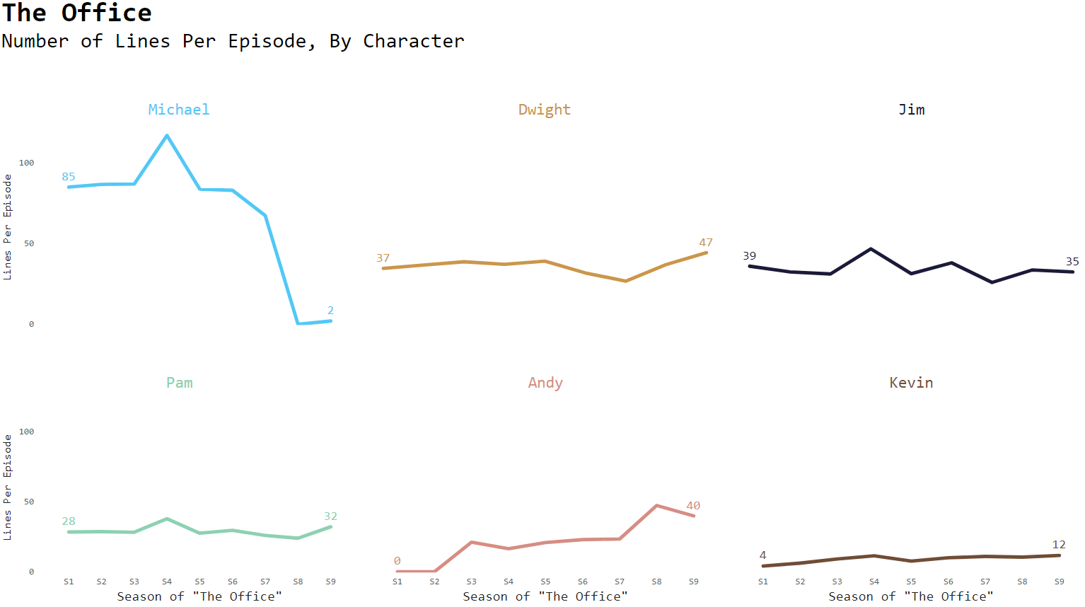
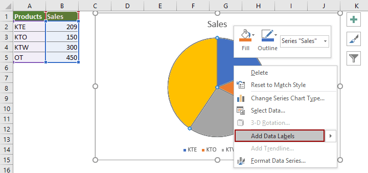
› teachersTeaching Tools | Resources for Teachers from Scholastic Flip Charts Games & Manipulatives Pocket Charts Poster Sets Storage & Organization Supplies Professional Growth Downloadable Book PDFs ... Add / Move Data Labels in Charts - Excel & Google Sheets Add and Move Data Labels in Google Sheets Double Click Chart Select Customize under Chart Editor Select Series 4. Check Data Labels 5. Select which Position to move the data labels in comparison to the bars. Final Graph with Google Sheets After moving the dataset to the center, you can see the final graph has the data labels where we want. Directly Labeling in Excel - Evergreen Data There are two ways to do this. Way #1 Click on one line and you'll see how every data point shows up. If we add a label to every data points, our readers are going to mount a recall election. So carefully click again on just the last point on the right. Now right-click on that last point and select Add Data Label. THIS IS WHEN YOU BE CAREFUL. Add or remove data labels in a chart - Microsoft Support Click the data series or chart. To label one data point, after clicking the series, click that data point. In the upper right corner, next to the chart, click Add Chart Element > Data Labels. To change the location, click the arrow, and choose an option. If you want to show your data label inside a text bubble shape, click Data Callout.
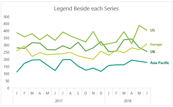
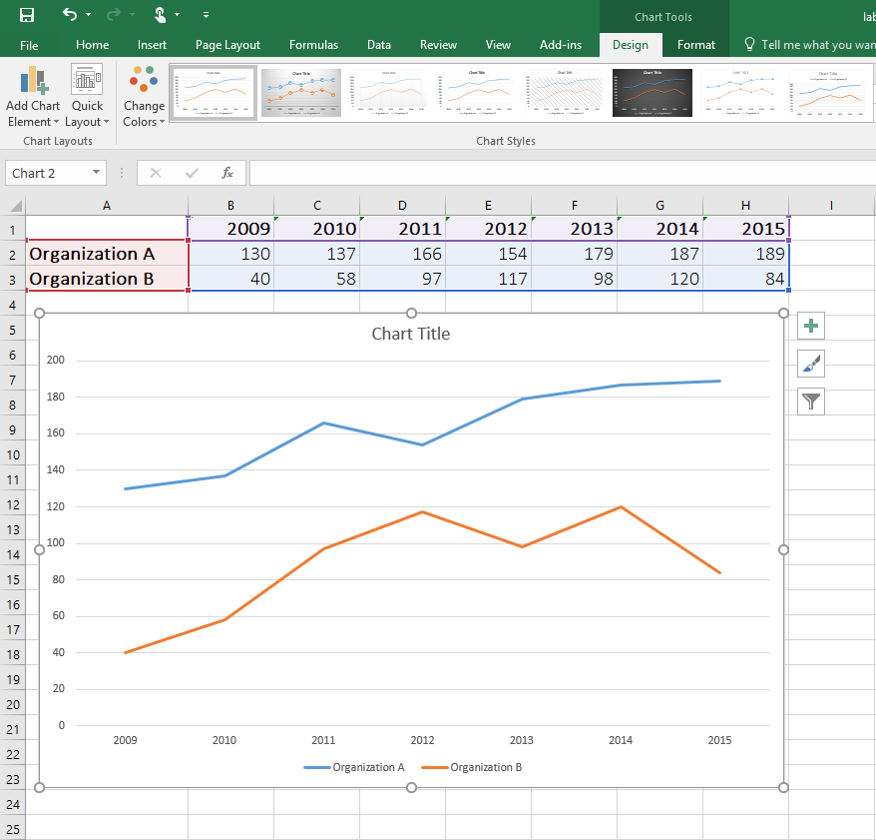
Edit titles or data labels in a chart - Microsoft Support On a chart, click one time or two times on the data label that you want to link to a corresponding worksheet cell. The first click selects the data labels for the whole data series, and the second click selects the individual data label. Right-click the data label, and then click Format Data Label or Format Data Labels. Creating a chart with dynamic labels - Microsoft Excel 365 For the existing chart (for example, see how to create a simple competition chart), do the following: Add the data series labels. 1. Select the data series, then do one of the following: Click on the Chart Elements button, select the Data Labels list, then select the position of the labels (the options depend on the data series chart type): How to Add Two Data Labels in Excel Chart (with Easy Steps) 4 Quick Steps to Add Two Data Labels in Excel Chart Step 1: Create a Chart to Represent Data Step 2: Add 1st Data Label in Excel Chart Step 3: Apply 2nd Data Label in Excel Chart Step 4: Format Data Labels to Show Two Data Labels Things to Remember Conclusion Related Articles Download Practice Workbook Excel Charts: Dynamic Label positioning of line series - XelPlus Select your chart and go to the Format tab, click on the drop-down menu at the upper left-hand portion and select Series "Budget". Go to Layout tab, select Data Labels > Right. Right mouse click on the data label displayed on the chart. Select Format Data Labels. Under the Label Options, show the Series Name and untick the Value.
A Complete Guide to Funnel Charts | Tutorial by Chartio
Data Labels in Excel Pivot Chart (Detailed Analysis) Add a Pivot Chart from the PivotTable Analyze tab. Then press on the Plus right next to the Chart. Next open Format Data Labels by pressing the More options in the Data Labels. Then on the side panel, click on the Value From Cells. Next, in the dialog box, Select D5:D11, and click OK.
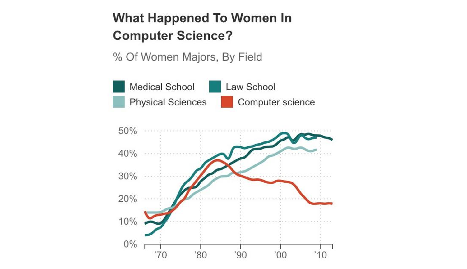
Directly Labeling Your Line Graphs | Depict Data Studio
How to Change Text or Label Direction in Excel Chart - YouTube In this video, you will learn how to change the direction of text or label in excel charts.
7 steps to make a professional looking line graph in Excel or ...
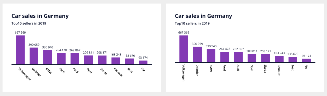
A complete guide to professional looking bar charts. — Vizzlo
Essential Chart Types for Data Visualization | Tutorial by ...
How To Add Start & End Labels in Power BI - Data Science ...
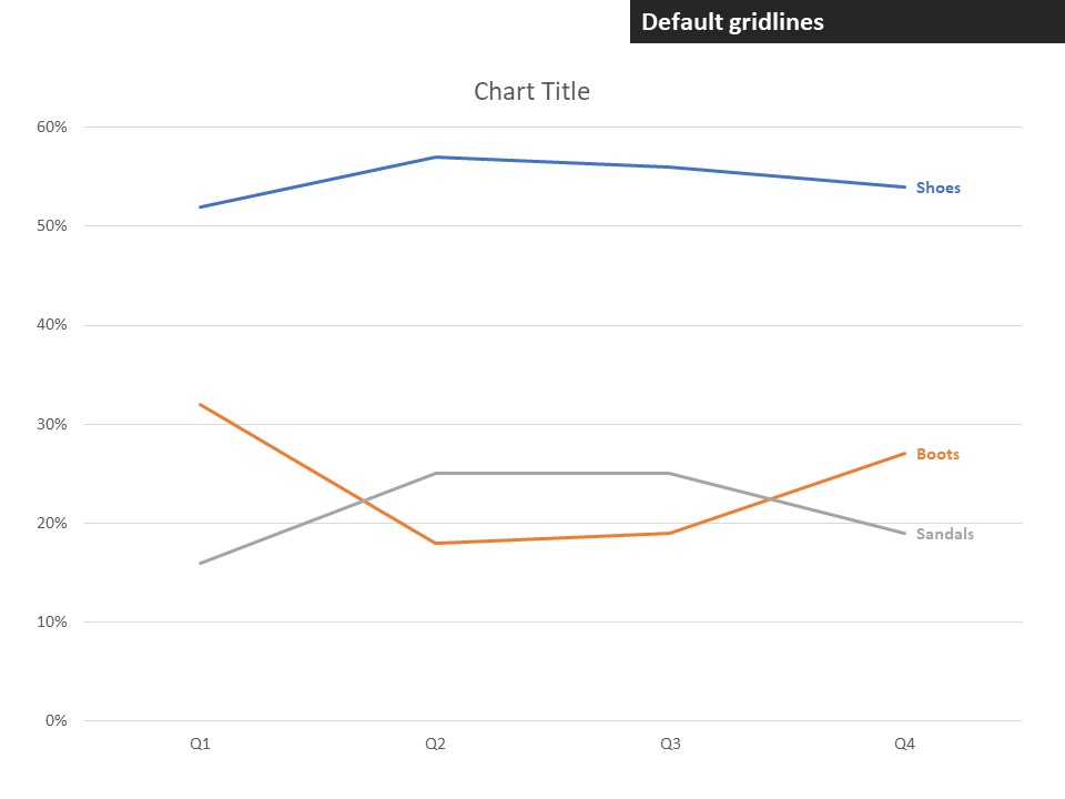
Label line chart series
Dynamically Label Excel Chart Series Lines • My Online ...

How to create a bi-directional bar chart in Excel?

Add label to Excel chart line • AuditExcel.co.za MS Excel ...
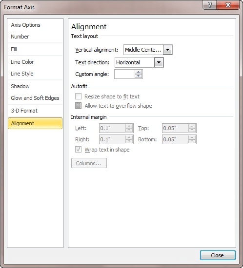
Adjusting the Angle of Axis Labels (Microsoft Excel)
How to add live total labels to graphs and charts in Excel ...
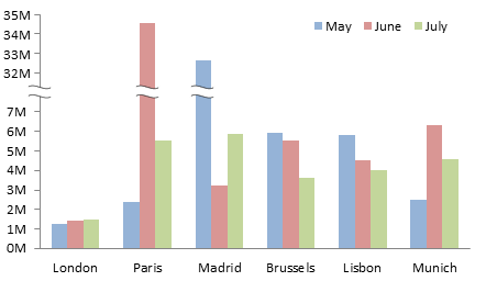
Broken Y Axis in an Excel Chart - Peltier Tech
EXCEL Charts: Column, Bar, Pie and Line
Changing Axis Tick Marks (Microsoft Excel)

Directly Labeling in Excel

How to Add Data Labels to an Excel 2010 Chart - dummies

424 How to add data label to line chart in Excel 2016
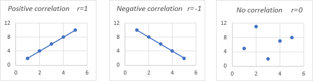
Correlation in Excel: coefficient, matrix and graph

Directly Labeling Your Line Graphs | Depict Data Studio
Best Types of Charts in Excel for Data Analysis, Presentation ...

How to use data labels in a chart

Microsoft Excel Charting Glossary Terms Definitions Examples ...

8 Ways To Make Beautiful Financial Charts and Graphs in Excel

How to Use Cell Values for Excel Chart Labels
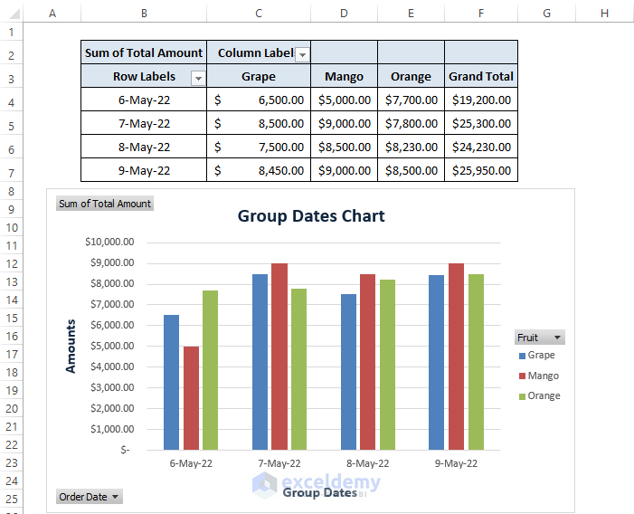
How to Group Dates in Excel Chart (3 Easy Ways) - ExcelDemy

Highlighting the difference between actual and target – User ...
Best Types of Charts in Excel for Data Analysis, Presentation ...
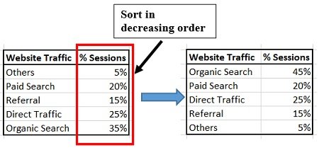
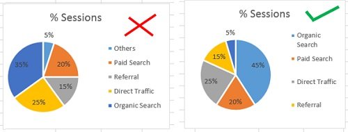
How to show percentage in pie chart in Excel?

Custom data labels in a chart
How to Add Data Labels to an Excel 2010 Chart - dummies
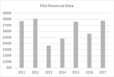
Revenue Chart Showing Year-Over-Year Variances - Peltier Tech

axis vs data labels — storytelling with data

Excel Charts: Dynamic Label positioning of line series
Sales Graphs And Charts - 35 Examples For Boosting Revenue
Creating Advanced Excel Charts: Step by Step Tutorial
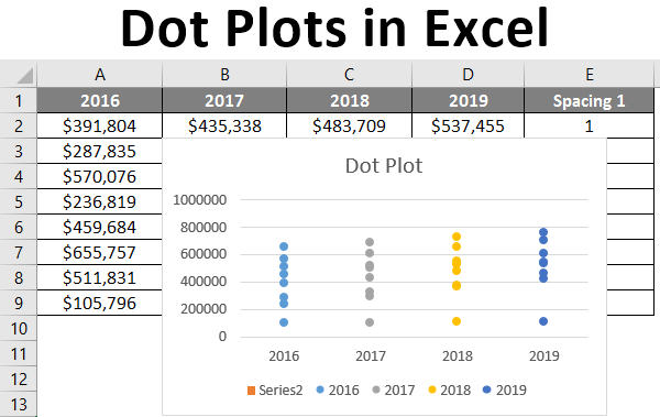
Dot Plots in Excel | How to Create Dot Plots in Excel?
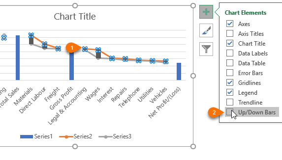
Excel Waterfall Charts • My Online Training Hub
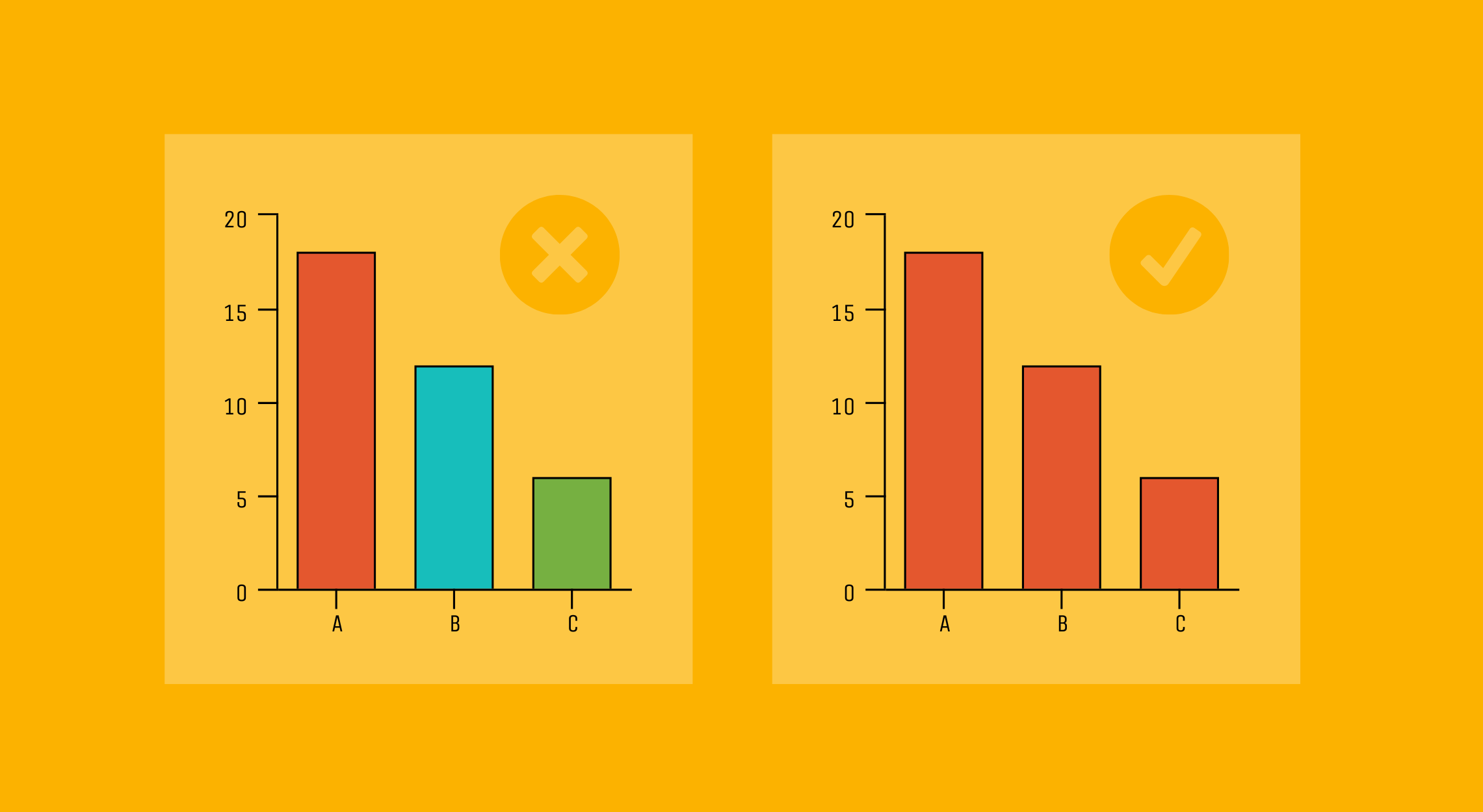
10 Do's and Don'ts of Infographic & Chart Design - Venngage
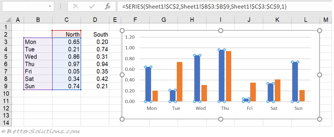
Excel Charts - Series Formula
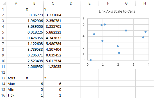
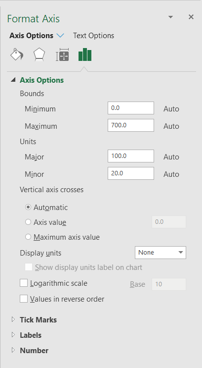
Link Excel Chart Axis Scale to Values in Cells - Peltier Tech

Directly Labeling in Excel

Data visualization - Material Design
How to Place Labels Directly Through Your Line Graph in ...
Clutter-Free: One of the 3 Cs for Better Charts
0 Response to "45 direct label excel charts"
Post a Comment